 MVLscope
HOW TEM WORKS
From electrons
to an image.
A transmission electron microscope sends electrons through a thin specimen. Follow the journey, change one thing, and see what reaches the camera.
Inside a transmission electron microscope
The source produces electrons in a vacuum. Condenser lenses shape the illumination. A thin specimen changes the electron wave through scattering. Objective and projection lenses form an enlarged image, which a detector records.
In bright-field imaging an objective aperture can exclude scattered electrons. Real contrast also depends on material, diffraction and phase. In diffraction mode, the imaging system projects the objective back focal plane instead of its image plane.
The interactive controls will appear when ready. If they do not load, the explanation and sources below remain available.
Explore TEMlabCHAPTER 01 / 06
A source, a path, a signal.
What reaches the camera
Patterned model foil
Same material, different thicknessLet the beam through
Follow the path
See the whole column ↓UNDERSTAND THE CHANGE
What changed?
Look for this
Describe the current view
PAUSE & PREDICT · OPTIONAL
Inside the column Hardware, beam and image paths
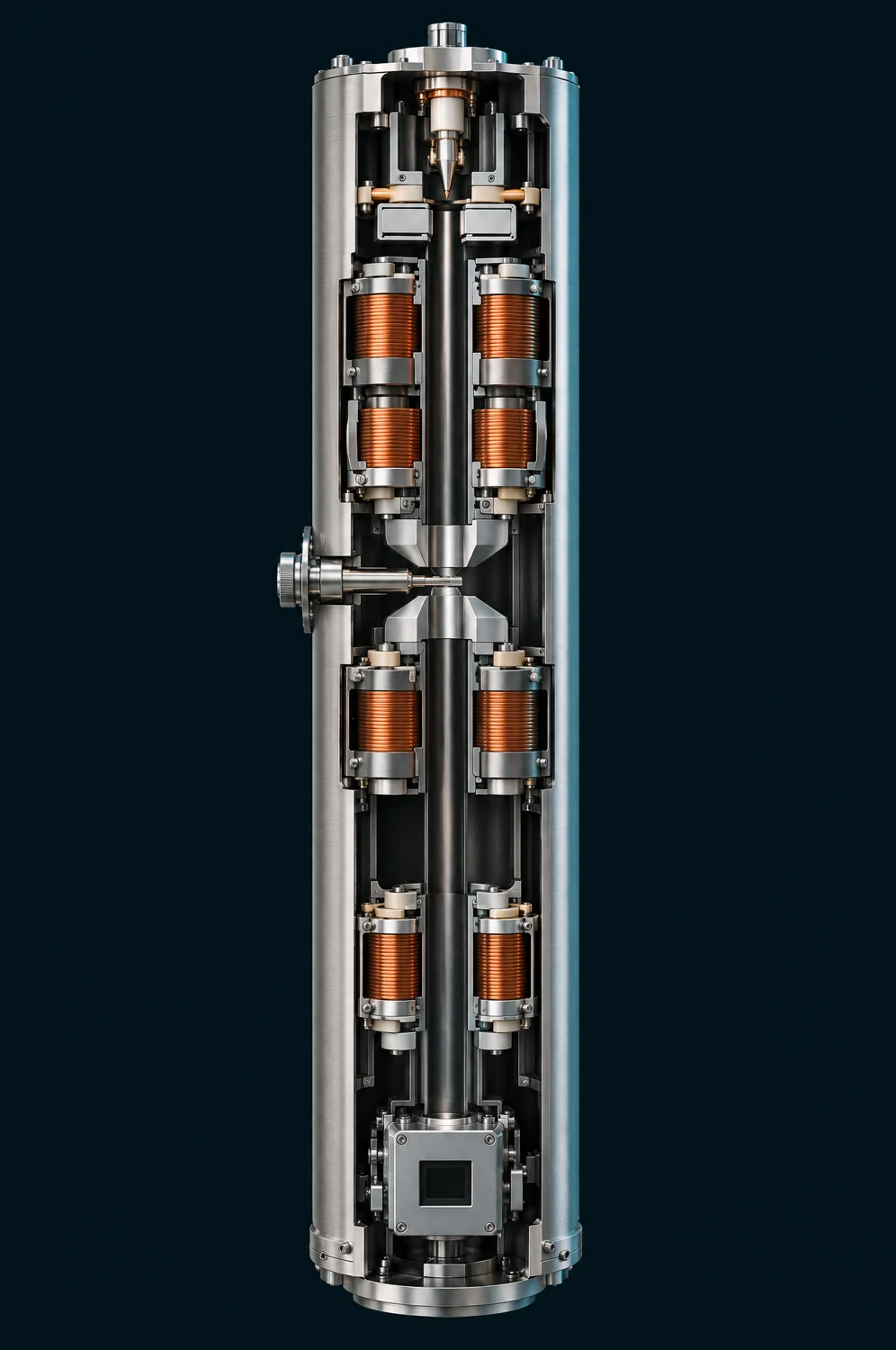 Image plane selected
Preparing the cutaway…
Follow the electron column
Explore the source, the thin specimen and the magnetic lenses that guide the signal to the camera.
Illustrative cutaway · paths and planes are teaching overlays.
Schematic paths · not to scale. Dots follow illumination to the specimen.
Column parts, in order
- Source and beam blanker
- Condenser: shapes illumination
- Thin specimen
- Objective: forms two planes
- Back focal plane: directions
- Image plane: specimen positions
- Intermediate and projector: relay a plane
- Camera: records that plane
TAKE THE IDEA INTO THE LAB
You have followed the signal.
Now explore these ideas using the controls in TEMlab. Change one setting, watch the image, and use the video lesson if you want an example.
Meet the instrument · TEM
A column enclosure hides the lenses and imaging planes shown in this lesson.
Go deeper: science, assumptions and sources
One useful example, with clear limits
The first five chapters use an invented foil with regions of the same material but different thickness. It is a simplified bright-field scattering-loss example. Real TEM images can retain contrast with the objective aperture out; this model deliberately omits those additional mechanisms. It omits phase contrast, crystal diffraction contrast, multiple-scattering detail, aberration correction, noise, detector efficiency and damage. Darker does not uniquely mean thicker in a real TEM.
The displayed signal is I = I₀ exp[−τ(1−A)], where τ is a relative scattering thickness and A is the model fraction of angles accepted by the objective aperture. Electrons excluded from the image are not necessarily absorbed: many have passed through the specimen at a different angle. The electron-balance description refers to the crosshair point, not the whole camera image.
The two-bar condenser system represents coordinated illumination, not one calibrated lens control. Its beam width at the final lens can change as the illumination setting changes. The drawing uses one fixed spatial scale without clipping its envelope. The condenser envelope has a finite waist: σ² = σ₀² + α²(z−z₀)². Illumination is a normalized Gaussian with constant total current over the full plane. Spreading lowers current density; some current can lie outside the displayed field. A fixed tone curve reveals both spread and concentrated illumination without changing the underlying current: greyscale display value = √[ln(1 + I/0.1) / ln(201)], with the same constants for all foil views. The greyscale display value is therefore nonlinear, not a calibrated electron count. The specimen ring marks one Gaussian width (σ); light also falls outside it. Blanking diverts illumination while leaving the source on. Vacuum is assumed ready throughout; this is not a pump-down or valve-operating procedure.
Focus is represented by a normalized Gaussian blur around a reference plane. The focus control is labelled by lens strength (stronger / weaker), not a signed instrument defocus convention. Its description compares the displayed central-gap contrast with that chapter’s reference image; it is not a resolution measurement. It is not a TEM contrast-transfer function or a claim that zero defocus is always best. A very small objective aperture also adds illustrative diffraction blur. Blur uses edge extension at the boundary. Screen enlargement resamples the same image; it does not introduce additional information or change the electron optics.
Hardware appearance is illustrative; calculated rays share the lesson model. Magnetic lenses are shown as coils and pole pieces. Displayed planes are not screens.
Two planes, one specimen
Chapter 6 deliberately switches to an ideal, periodic amplitude specimen. Illumination is uniform and the objective aperture is out in this separate example. Its image is |ψ|² and its diffraction distribution is |FFT(ψ)|², with real positive exit-wave amplitude ψ and no phase term. The diffraction intensity uses ln(1 + I), divided by its fixed reference maximum, to reveal weaker spots. It is displayed as a labelled 2× central crop with nearest-neighbour sampling. The periodic image uses a linear display of |ψ|². These different display curves do not alter the calculated intensity or FFT. It is not an image FFT, an atomic-resolution crystal calculation, or a prediction for the earlier foil. The repeated features and Fourier field are dimensionless.
The objective forms an image plane and a back focal plane at the same time. Changing the intermediate-lens setting selects which plane is relayed to the camera. The diagram uses consistent paraxial thin-lens rays above the relay. In the focus chapter the image and angle planes remain at their reference positions while lens strength changes. The few drawn rays illustrate selected directions; they are not an electron count. Below that, dashed arrows indicate plane selection, not a calibrated multi-lens ray trace. The camera stays in place. The first five camera views are turned 180° from the specimen thumbnail, consistent with the drawn objective image. The marked crosshairs show the same foil point. Real instruments can further rotate or invert their final images. The periodic example is centrosymmetric, so its image orientation is unchanged in appearance.
The marked foil point and its thickness are illustrative; specimen thumbnails use colour to show relative thickness. Camera images are greyscale. Animated dots are a way to follow a path, not tracked individual quantum trajectories or actual electron speeds. Motion starts only when requested. With reduced motion enabled, the button advances one still step instead of running an animation. Dots follow only the illumination path to the specimen.
Scientific reading
- Indiana University — Beam current, illuminated area and current density
- University of Iowa — Condenser illumination and objective focus
- Indiana University — Objective aperture, contrast and resolution
- ETH Zürich — Fourier relationship at the back focal plane
- JEOL — Transmission electron microscope basics
- JEOL — Condenser lenses
- JEOL — Imaging lens system
- ETH Zürich — Bright-field TEM
- ETH Zürich — Image and diffraction plane selection
- JEOL — Phase contrast transfer